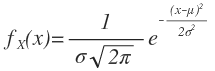
Python을 이용해 정규분포를 그려보려 한다. 정규분포의 pdf는 다음과 같다.
1. 직접 생성
위 식을 함수로 정의하면, 다음과 같다
import matplotlib.pyplot as plt
import math

def normal_pdf(x, mu=0, sigma=1):
    return(math.exp(-(x-mu)**2)/(2*sigma**2))/(math.sqrt(2*math.pi)*sigma)
다음과 같이 xs_1에 대한 정규분포를 구해보자(plot에 정수값을 넣을 수 없으므로, x/10을 대입)
xs_1 = [x/10 for x in range(-50, 50)]
plt.plot(xs_1, [normal_pdf(x) for x in xs_1])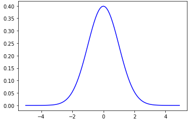
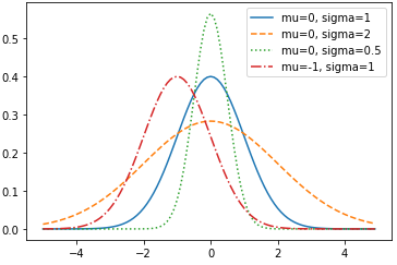
다양한 정규분포를 구해보면,
plt.plot(xs, [normal_pdf(x, sigma=1) for x in xs], '-', label='mu=0, sigma=1')
plt.plot(xs, [normal_pdf(x, sigma=2) for x in xs], '--', label='mu=0, sigma=2')
plt.plot(xs, [normal_pdf(x, sigma=0.5) for x in xs], ':', label='mu=0, sigma=0.5')
plt.plot(xs, [normal_pdf(x, mu=-1) for x in xs], '-.', label='mu=-1, sigma=1')
plt.legend()
plt.title('Gaussian CDF')
평균값이 동일할 때,
표준편차가 커지면 최댓값은 작아지고 옆으로 넓게 퍼진 그래프가 나타난다
반대로 표준편차가 작아지면 최댓값은 커지고 좁게 퍼진 그래프가 나타난다
2. scipy.stats의 norm 사용
scipy 라이브러리에 있는 scipy.stats.norm.pdf를 이용하면 미리 정의되어 있는 정규분포의 pdf를 이용할 수 있다. scipy의 함수는 numpy의 ndarray값을 입력으로 받을 수 있어 매우 유용하다.
import numpy as np
import scipy.stats as st
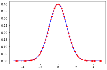
xs_2 = np.arange(-5, 5, 0.1)
plt.plot(xs_2, st.norm.pdf(xs_2, loc=0, scale=1), 'r+')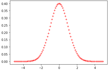
둘을 동시에 플롯하면 완전히 일치함을 볼 수 있다
'DataScience' 카테고리의 다른 글
| 조건부 확률 (Conditional Probability) (0) | 2020.09.08 |
|---|---|
| 오차함수와 정규분포와의 관계 (0) | 2020.09.02 |
| 정규분포의 정의와 평균, 분산 (0) | 2020.09.02 |
| [Matplotlib] 한글 폰트 설정, 글꼴 변경 (4) | 2020.08.29 |
| [Matplotlib] 개요 (0) | 2020.08.26 |